XOR problem

In learning a new field I don't think an introduction using the most basic example doesn't help. Using the XOR problem to understand deep learning often obscures the grander picture. That being said, I'm not sure who this explanation is for. At the moment, myself. Why? To see how well I can explain the fundamental concepts of deep learning using a toy example.

A quick history lesson.

Perceptrons are functions that perform a linear operation followed by a non linear function mapping. In general, taking inputs $x_1, x_2, ..., x_n$ to an output $f(\sum_i^n {w_i x_i})$. Letting $f(z)$ be a step function with value 1 if z > 0 else 0.

The problem here is that we are only able to find functions that are linearly separable.

Multilayer and differentiable activation functions

What we want to do is add non linearity to our input. By doing so we can transform our feature space for a linear model to learn.

The architecture

The network consists of two inputs $x_1$ and $x_2$, a hidden layer $\textbf{h}= [h_1, h_2]$ and output $y$.

Task

Find the parameters (weights) $\theta$ that minimize the error (loss) between estimated function $f$ and our estimate $f^*$. We want our $\theta$ values to produce an estimate as close to $f^*$ as possible, or for the loss function $\mathcal L$ to be as close to zero.

The mean squared error

$$\mathcal L(\theta) = \frac{1}{2} \sum_{x} (f^*(\textbf{x}) - f( \textbf{x} ; \theta))^2$$

has a nice derivative

$$\nabla{\mathcal L_{\theta}} = \sum_{x} (f^*(\textbf{x}) - f( \textbf{x} ; \theta)) \nabla f( \textbf{x} ; \theta).$$

(i.e. the product of the summed difference and the change in our estimated function $f(\textbf{x}; \theta)$ with respect to a change in $\theta$)

Optimization, Gradient Descent

In thinking of our loss function as a terrain, we want the coordinates that reaches the lowest valley.

We start at coordinates $\theta_0$ and ask, how do we find the deepest valley? Intuitively, a natural step would to go in the direction with the steepest incline by a small $\alpha$ sized step, $-\alpha \nabla_{\theta}{\mathcal L}$.

Taking the step, we arrive at a new coordinate $\theta_1$. Repeating this process choose the direction with the steepest decline until we reach our destination

$\theta_{n+1} = \theta_{n} - \alpha \nabla_{\theta}{\mathcal L}$.

Backpropagation

Going back to the XOR problem we have

$$\textbf{x} \rightarrow f(\textbf{W}^T\textbf{x}) = \textbf{h}$$

$$\textbf{h} \rightarrow g(\textbf{w}^T \textbf{h}) \rightarrow \textbf{w}^T f(\textbf{W}^T\textbf{x} ) = y.$$

The parameter $\theta$ is made up of different weights $\textbf W$ and $\textbf w$ that the network will need to learn.

Thus

$$\begin{aligned} \nabla_{x} \mathcal L &= \frac{\partial \mathcal L}{\partial y} \\ &= \frac{\partial y}{\partial (\textbf w^T \textbf h)} \\ &= \frac{\partial (\textbf w^T \textbf h)}{\partial h} \\ &= \frac{\partial h}{\partial (\textbf W ^T \textbf x)} \\ &= \frac{\partial (\textbf W^T \textbf x)}{\partial x} \end{aligned}$$

$$(y - y^*) \textbf w f'(.) \textbf W$$

where y is our predicted value, $y^*$ is the true value.

$$\nabla_{w} \mathcal L = \frac{\partial \mathcal L}{\partial y} \frac{\partial y}{\partial (\textbf w^T \textbf h)} \frac{\partial (\textbf w^T \textbf h)}{\partial \textbf w} = (y - y^*) \textbf h $$

and

$$\begin{aligned} \nabla_{W} \mathcal L &= \frac{\partial \mathcal L}{\partial y} \frac{\partial y}{\partial (\textbf w^T \textbf h)} \frac{\partial (\textbf w^T \textbf h)}{\partial h} \frac{\partial h}{\partial (\textbf W ^T \textbf x)} \frac{\partial (\textbf W^T \textbf x)}{\partial W} \\ &= (y - y^*) \textbf w f'(\textbf W ^T \textbf x)\textbf x \end{aligned}$$

$$\frac{\partial \mathcal L}{\partial y} = (y - y^*)$$

$$\frac{\partial (\textbf w^T \textbf h)}{\partial h} = \textbf w$$

$$\frac{\partial h}{\partial (\textbf W ^T \textbf x)} = f'(\textbf W ^T \textbf x)$$

$$\frac{\partial (\textbf W^T \textbf x)}{\partial x}= \textbf W$$

Activation Function

The most common non-linear function used in modern neural networks is the ReLU

$$f(z) = \max(0, z)$$

or variations of it.

Its derivative

$$f'(z) = \max(0, 1)$$

is easy to compute even though it is non differentiable at 0.

The sigmoid function

$$g(z) = \frac{1}{1 + \exp(-z)}$$

is used in binary classification problems with derivative

$$g'(z) = g(z)(1 - g(z))$$

Numpy Implementation

import numpy as np

>>> X = np.array([[0, 0], [0, 1], [1, 0], [1, 1]])
>>> Y = np.array([[0], [1], [1], [0]])
>>> print(" A  B | XOR(A,B)")
>>> print("-----------------")
>>> for i, bits in enumerate(X):
...     print(f" {bits[0]}  {bits[1]} |     {Y[i][0]}")

 A  B | XOR(A,B)
-----------------
 0  0 |     0
 0  1 |     1
 1  0 |     1
 1  1 |     0

def sigmoid(x):
    """ non-linear function """
    return 1.0 / (1.0 + np.exp(-x))

def dx_sigmoid(x):
    return sigmoid(x) * (1. - sigmoid(x))

def relu(x):
    return np.maximum(0, x)

def dx_relu(x):
    return x * (x > 0)

def loss_fn(predicted, true):
    return 0.5 * (predicted - true) ** 2

# 100 iterations 
iterations = 10000

input_dim = X.shape[-1]
output_dim = Y.shape[-1]
lr = 0.1 # learning rate

hidden_dim = 2
W = np.random.uniform(size=(input_dim, hidden_dim))
w = np.random.uniform(size=(hidden_dim, output_dim))

activation_fn = relu
dx_activation_fn = dx_relu


>>> for step in range(1, iterations+1):
...    # forward pass
...
...    # (4, 2) x (2, 2) -> (4, 2)
...    fc1 = X.dot(W)
...    # (4, 2)
...    hidden = activation_fn(fc1)
...    # (4, 2) x (2, 1) ==> (4, 1)
...    output = hidden.dot(w)
...
...    loss = loss_fn(output,  Y)
...    if step % 1000 == 0:
...        print(f"Loss: {np.mean(loss):.6f}  Step: {step}/{iterations}")
...
...    ## backward pass 
...    #(4x1)
...    error = output - Y
...
...    delta_hidden = error.dot(w.T) * dx_activation_fn(fc1) 
...
...    ## gradient descent
...
...    grad_w = hidden.T.dot(error)
...    w -= lr * grad_w
...
...    grad_W = X.T.dot(delta_hidden)
...    W -= lr * grad_W



Loss: 0.000012  Step: 1000/10000
Loss: 0.000003  Step: 2000/10000
Loss: 0.000001  Step: 3000/10000
Loss: 0.000001  Step: 4000/10000
Loss: 0.000000  Step: 5000/10000
Loss: 0.000000  Step: 6000/10000
Loss: 0.000000  Step: 7000/10000
Loss: 0.000000  Step: 8000/10000
Loss: 0.000000  Step: 9000/10000
Loss: 0.000000  Step: 10000/10000

>>> for i, prediction in enumerate(output):
...    print(f'predicted {prediction[0]:.5f} => true {Y[i][0]}')

predicted 0.00000 => true 0
predicted 1.00000 => true 1
predicted 1.00000 => true 1
predicted 0.00084 => true 0

>>> print(W)

array([[-0.85018314,  0.80808135],
       [ 0.85056309, -0.80776054]])

>>> print(w)

array([[1.1756913 ],
        [1.23749876]])

plot

from matplotlib import pyplot as plt
from mpl_toolkits.mplot3d import Axes3D
from matplotlib import cm

def xorNet(x):
    fc1 = x.dot(W)
    hidden = relu(fc1)
    out = hidden.dot(w)
    return out

xx, yy = X[:,0], X[:,1]
z = Y.T[0]

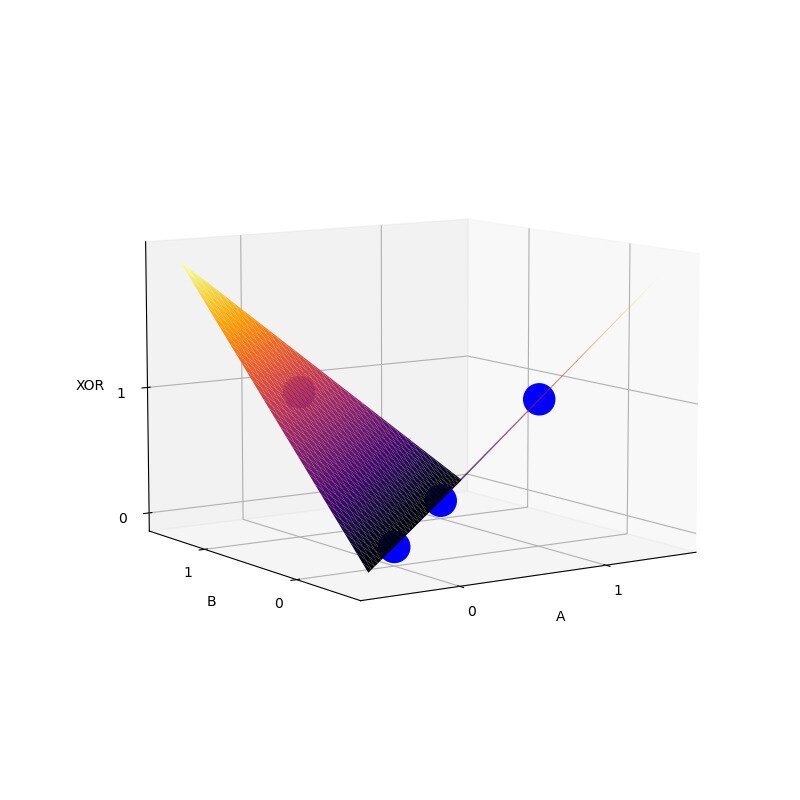
def splot(ax3d, nticks=101):
    """surface plot of the xor outputs of
    the self.net for a mesh grid inputs of a and b:"""
    i = np.linspace(-0.5,1.5,nticks)
    a,b = np.meshgrid(i,i)
    ab = np.stack([a,b],axis=-1)
    xor = xorNet(ab)
    xor.shape = (nticks,nticks)
    ax3d.clear()
    fn = ax3d.plot_surface(a,b,xor,cmap='inferno',)#edgecolor='none')
    ax3d.view_init(elev=30,azim=-60)
    ax3d.set_xticks([0,1]),ax3d.set_xlabel('A')
    ax3d.set_yticks([0,1]),ax3d.set_ylabel('B')
    ax3d.set_zticks([0,1]),ax3d.set_zlabel('XOR')

    plt.draw()
    plt.pause(0.05)

fig = plt.figure(figsize=(8,8))
ax3d = plt.axes(projection='3d')
splot(ax3d)
ax3d.scatter(xx, yy, z, color= "blue", s=500, marker='o', alpha=1)
plt.show()

xor-relu-soln