Data Description and Background
Public Transport Journeys by Type of Transport
The data set comes from the Transport for London website. It describes the number of journeys on the public transport network by TFL reporting period, by type of transport. Data is broken down by bus, underground, DLR, tram, Overground and cable car.
Some information about the dataset from the data description:
Period lengths are different in periods 1 and 13, and the data is not adjusted to account for that. Docklands Light Railway journeys are based on automatic passenger counts at stations. Overground and Tram journeys are based on automatic on-carriage passenger counts. Reliable Overground journey numbers have only been available since October 2010.
In this project we will be forecasting the number of journeys on the London Underground network.
We first create a test set the last 5 journey counts on the London Underground network to compare with our final forecasts.
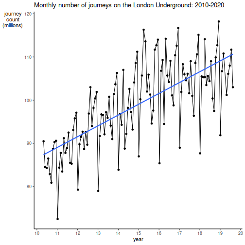
Visualise the time series plot
## `geom_smooth()` using formula 'y ~ x'
##                  Estimate   Std. Error  t value     Pr(>|t|)
## (Intercept)  4.983828e+03 4.579668e+02 10.88251 1.315793e-19
## period.start 6.840706e-03 6.413333e-04 10.66638 4.340164e-19
From the initial plot, we can see the time series is non-stationary. We also confirm this from the non-zero linear model regression coefficient.
We also notice seasonal patterns which we will discuss later.
Stationarity
After first order differencing we plot the time series, its autocorrelation and partial auto correlation plots.
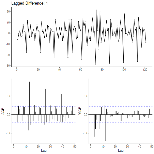
From the autocorrelation-lag plot we see high correlation at periodic intervals implying seasonality.
Seasonality
From the data we see months with two entries hence correlation every 13 lags. The data description also confirms this:
Period lengths are different in periods 1 and 13, and the data is not adjusted to account for that.
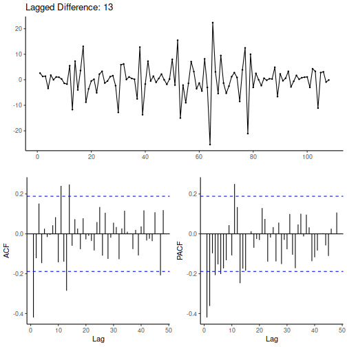
After applying differencing every 13 lags we see a clearer representation of the ACF and PACF plots. We initially consider ARIMA(0,1,1)(0,1,1)[13].
##
##  Ljung-Box test
##
## data:  Residuals from ARIMA(0,1,1)(0,1,1)[13]
## Q* = 5.4208, df = 8, p-value = 0.7118
##
## Model df: 2.   Total lags used: 10
##
## Call:
## arima(x = lu, order = c(0, 1, 1), seasonal = list(order = c(0, 1, 1), period = 13),
##     method = ("ML"))
##
## Coefficients:
##           ma1     sma1
##       -0.8258  -0.9033
## s.e.   0.0575   0.2643
##
## sigma^2 estimated as 16.43:  log likelihood = -314.98,  aic = 635.95
The model summary seems promising, we now check if the model is adequate using Ljung-Box tests for \(K = 6\), 12 and 24
##
##  Box-Ljung test
##
## data:  model1$residuals
## X-squared = 1.9491, df = 6, p-value = 0.9243
##
##  Box-Ljung test
##
## data:  model1$residuals
## X-squared = 14.991, df = 12, p-value = 0.242
##
##  Box-Ljung test
##
## data:  model1$residuals
## X-squared = 28.14, df = 24, p-value = 0.2542
From the Ljung-Box tests, we can conclude the model is adequate up to lag 24.
Overdifferencing
We now try to overfit the model. We start by increasing the degree of the seasonal moving average part to 4. Assuming quarterly seasonal variation.
##
##  Ljung-Box test
##
## data:  Residuals from ARIMA(0,1,1)(0,1,4)[13]
## Q* = 5.4319, df = 5, p-value = 0.3655
##
## Model df: 5.   Total lags used: 10
##
## Call:
## arima(x = ts(lu), order = c(0, 1, 1), seasonal = list(order = c(0, 1, 4), period = 13),
##     method = ("ML"))
##
## Coefficients:
##           ma1     sma1     sma2     sma3    sma4
##       -0.8087  -0.8449  -0.0553  -0.2369  0.2667
## s.e.   0.0634   0.3447   0.1598   0.1669  0.1404
##
## sigma^2 estimated as 14.78:  log likelihood = -311.11,  aic = 634.21
A decrease in AIC by 1.74, decrease in log likelihood by 3.87 suggesting this model is a better fit to our data.
We now consider ARIMA(0,1,2)(1,1,4)[13].
##
##  Ljung-Box test
##
## data:  Residuals from ARIMA(0,1,2)(0,1,4)[13]
## Q* = 5.676, df = 4, p-value = 0.2247
##
## Model df: 6.   Total lags used: 10
##
## Call:
## arima(x = lu, order = c(0, 1, 2), seasonal = list(order = c(0, 1, 4), period = 13),
##     method = ("ML"))
##
## Coefficients:
##           ma1      ma2     sma1     sma2     sma3    sma4
##       -0.7609  -0.0592  -0.8321  -0.0662  -0.2256  0.2670
## s.e.   0.1020   0.1022   0.2908   0.1589   0.1660  0.1458
##
## sigma^2 estimated as 14.85:  log likelihood = -310.94,  aic = 635.87
No improvement in the reduction of the log likelihood or AIC.
The AIC is slightly higher compared to ARIMA(0,1,1)(0,1,4)[13].
We conclude that ARIMA(0,1,1)(0,1,4)[13] is the best fitted model to the data.
Forecasting
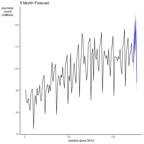
Comparing with the test data we see all points lie close to the point forecast.
Conclusion
From the analysis, we can see the yearly growth of the London Underground network usage.
We note there is seasonal effects of the number of journeys on the London Underground network each year.
We first fit the data to an ARIMA(0,1,1)(0,1,1)[13] and after overdifferencing concluded that a ARIMA(0,1,1)(0,1,4)[13] was more suitable.
We then forecasted the next 5 months resulting in accurate forecasts. All of which lie in the 80% forecast interval.